Expectation-Maximization (EM) Algorithm and application to Belief Networks

The EM algorithm is a versatile technique for performing Maximum Likelihood Estimation (MLE) under hidden variables. In this post, we will go over the Expectation Maximization (EM) algorithm in the context of performing MLE on a Bayesian Belief Network, understand the mathematics behind it and make analogies with MLE for probability distributions. An accompanying Python (NumPy) implementation is available on GitHub:

View on GitHub

When EM algorithm can be used

EM algorithm comes in handy when (1) an analytical solution for MLE (i.e. using derivatives) is not possible and/or (2) in the case of missing data. Recall that we can find the Maximum Likelihood estimates for commonly used probability distributions (e.g. Gaussian, Poisson and Binomial) analytically. There exist very standard formulas for finding the ML estimates of their parameters (mean and variance in case of Gaussian for example). If your concepts regarding Maximum Likelihood estimation are not clear, I greatly recommend this read.

In the case of probability matrices however, we need to take an iterative approach, since each cell of these matrices can be considered a parameter, and we don’t quite know what this parameter represents. Gaussian distribution for example, we know, has mean and variance as it’s parameters.

Just like the ML estimates of probability distribution parameters, the ML estimates of probability matrices are also a function of the training data. We need to find the probability distributions (which may be in the form of probability matrices) that maximize the likelihood of this data.

Application to Bayesian Belief Networks

EM algorithm is applied in a variety of situations. In this article, we will go over examples involving Bayesian Belief Networks. A lot of problems can be modeled as Bayesian Belief Networks, hence making this a great example. Bayesian Belief Networks are one of the two types of probabilistic graphical models (the other being Markov Random Fields). Since Bayesian Belief Networks are directed and acyclic, they are simpler to model mathematically. This article does not assume knowledge of Bayesian Belief Networks, however, if you would like to learn more, I found [1] an excellent reference.

Derivation

Despite being more numerical than analytical, EM algorithm cannot be understood without delving into the mathematics behind it. We show the derivation for discrete random variables. With minor modifications, the same can be applied to continuous random variables as well by using integrals instead of summations.

Notation

Let’s start with the notation to make our lives easy:

• Upper case letters will denote random variables and
• Their lower case equivalents will denote specific values that they may take
  • Example: \(P(D=d \mid A=a, B=b)\) means the probability of random variable \(D\) taking the value \(d\) provided \(A\) and \(B\) are \(a\) and \(b\) respectively.
  • As a shorthand, we may skip the upper case. For example, \(P(d \mid a, b)\) means \(P(D=d \mid A=a, B=b)\)

The term variable and node (of the Belief Network) may be used interchangeably. Also, a vector is a 1-D tensor and a matrix is a 2-D tensor.

For each node (or random variable) \(i\) in the graph, we will have:

• A true PMF \(P_i\) (from which we will sample training data). For example, \(P_D\) means \(P(D \mid A, B)\) for the graph in the following section.
  • Consequently, \(P\) is the joint PMF (of all the nodes).
• A variational PMF \(Q_i\) (more on this later).
  • Consequently, \(Q\) is the variational joint PMF (of all the nodes).
• An estimated PMF \(\hat{P}_i\) (which we will estimate from the sampled data). For example, \(\hat{P}_D\) means \(\hat P(D \mid A, B)\) for the graph in the following section.
  • Consequently, \(\hat{P}\) is the estimated joint PMF (of all the nodes).
• \(\lvert . \rvert\) will be used to refer to the number of states a random variable may take, e.g. \(\lvert A \rvert = 3\) means the random variable \(A\) can take one of 3 possible states

Analogy between \(\hat{P}\) and \(P(... \mid \theta)\)

In the Bayesian approach, the parameter itself is a random variable (represented by upper case \(\Theta\)) with a prior distribution. Ideally we would like to take this prior distribution into account at all times, however, since that isn’t always possible, we use estimates like Maximum Likelihood (ML) estimate or Maximum A Posteriori (MAP) estimate.

Maximum Likelihood estimation as you must have seen usually involves finding a value for this \(\Theta\), i.e. \(\theta_{\text{ML}}\) that maximizes a probability \(P(x \mid \theta)\) where \(\theta = \theta_{\text{ML}}\). This \(\Theta\) may be a single parameter or a set of parameters (\(\Theta\) for a Gaussian distribution, for example has two components, mean and variance, which we may call \(\Theta_1\) and \(\Theta_2\)).

The objective of the EM algorithm is not much different. Since we will be dealing with probability matrices, we will not have a single value \(\theta\) (or a few values e.g. \(\theta_1\), \(\theta_2\)) to estimate, rather, we’ll have a whole probability matrix to estimate, as seen in the next section. We may look at this matrix to estimate as a single joint PMF \(\hat{P}\) or a set of conditional PMFs \(\hat{P}_i\).

An estimated PMF may be represented as either \(\hat{P}\) or \(P(... \mid \theta)\) (both notations are similar). \(\hat{P}\) is a (estimated) parameter matrix where \(\theta\) refers to the parameters (values of this matrix). For example, \(\hat{P}(d \mid a, b)\) essentially means \(P(d \mid a, b, \theta)\). When the EM algorithm converges, we can say that our \(\theta = \theta_{\text{ML}}\) and the resulting \(\hat{P}\) tensor (or the set of \(\hat{P}_i\) tensors) will be the final result of the algorithm.

Problem Formulation

Let’s consider the following Bayesian Belief Network:

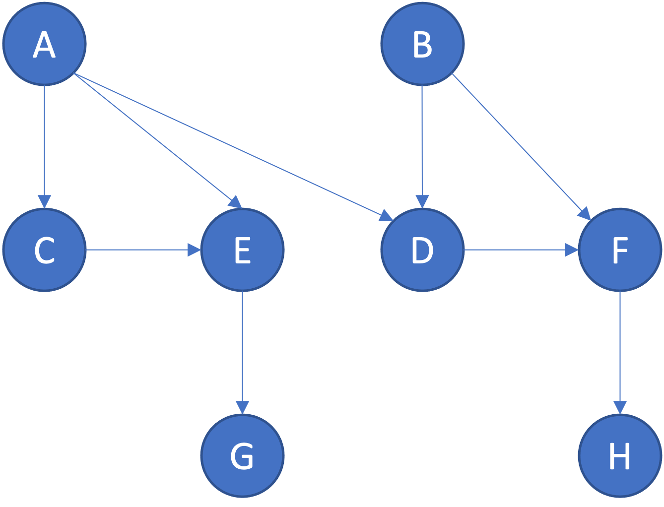
The nodes \(A\), \(B\), \(C\), \(D\), \(E\), \(F\), \(G\) and \(H\) represent random variables.

They may have any number of possible states. The PMF of the states a random variable may take depends on the states of it’s parent variables (if any). For example, the PMF of \(D\) depends on the states of \(A\) and \(B\). If a node does not have any parent variables, it’s PMF is simply a vector (i.e. 1-D tensor). Each parent variable adds a dimension to it’s PMF.

Training this Belief Network would look like estimating the PMFs of all its nodes, i.e. the PMF tensors \(\hat{P}(A)\) and \(\hat{P}(B)\) and the conditional PMF tensors \(\hat{P}(C \mid A)\), \(\hat{P}(D \mid A, B)\), \(\hat{P}(E \mid A, C)\), \(\hat{P}(F \mid B, D)\), \(\hat{P}(G \mid E)\) and \(\hat{P}(H \mid F)\), provided we have samples from true PMFs \(P(A)\), \(P(B)\), \(P(C \mid A)\), \(P(D \mid A, B)\), \(P(E \mid A, C)\), \(P(F \mid B, D)\), \(P(G \mid E)\) and \(P(H \mid F)\).

The dimensions of a probability matrix depend on the number of possible states of the random variable and it’s parents. For example:

\[P(D \mid A, B) \in \mathbb{R}^{\lvert D \rvert \times \lvert A \rvert \times \lvert B \rvert}\]

Provided the individual PMF tensors \(P_i\) (or \(\hat P_i\)) it’s easy to obtain the joint PMF \(P\) (or \(\hat P\)), or vice versa. Therefore, an alternative approach is to sample data directly from the joint PMF \(P\) and use that data to estimate the joint PMF \(\hat P_i\). We will discuss the pros and cons of both approaches. During analysis, we will use the joint PMFs as it makes the mathematics much simpler.

The objective of maximizing likelihood

Let’s suppose we have a single data point \((a_1, c_1, d_1, h_1)\) that represents the states of a subset of the variables (nodes) in the Belief Network you see above (e.g. consider \(A\), \(C\), \(D\) and \(H\) are known but \(B\), \(E\), \(F\) and \(G\) are not known).

The goal is to find a set of estimated probability matrices (\(\hat{P}_i\) for \(i \in \{A ... H \}\)) which maximize the (marginal) likelihood of the present (known) variables in this data point, i.e. maximize

\[P(A=a^1, C=c^1, D=d^1, H=h^1 \mid \theta)\]

The above is a marginal distribution of the present variables over the missing variables, a summation over all the possible values of \(B\), \(E\), \(F\) and \(G\).

Maximizing the likelihood is the same as maximizing the log-likelihood. Let’s use \(\ell (\theta)\) to denote the marginal log-likelihood of the present (known) variables for a single data point:

\[\ell (\theta) = \log P(A=a^1, C=c^1, D=d^1, H=h^1 \mid \theta)\]

Remember that \(P( ... \mid \theta)\) is essentially \(\hat{P}\). Maximizing the former over \(\theta\) is essentially finding the optimal \(\hat{P}\)

Also, \(\ell (\theta)\) expressed as a marginal is

\[\begin{align} \ell (\theta) &= \log P(A=a^1, C=c^1, D=d^1, H=h^1 \mid \theta) \\ &= \log \sum_{n=1}^{\lvert G \rvert} \sum_{m=1}^{\lvert F \rvert} \sum_{l=1}^{\lvert E \rvert} \sum_{k=1}^{\lvert B \rvert} P(A=a^1, B=b_k, C=c^1, D=d^1, E=e_l, F=f_m, G=g_n, H=h^1 \mid \theta) \end{align}\]

For simplicity in the next section, we simplify the above expression into

\[\begin{align} \ell (\theta) &= \log P(Y=y^1 \mid \theta) \\ &= \log \sum_{k=1}^{\lvert Z \rvert} P(Z=z_k, Y=y^1 \mid \theta) \end{align}\]

i.e., let \(Z\) represent all missing variables and \(Y\) represent all present variables.

Also, it should be remembered that this is the log-likelihood of just one data point. The log-likelihood over \(N\) data points is simply the sum of individual likelihoods. Let’s use \(\mathcal{L} (\theta)\) to represent it:

\[\begin{align} \mathcal{L} (\theta) &= \sum_{n=1}^{N} \log P(Y=y^n \mid \theta) \\ &= \sum_{n=1}^{N} \log \sum_{k=1}^{\lvert Z \rvert} P(Z=z_k, Y=y^n \mid \theta) \end{align}\]

However, be mindful that different data points may have different sets of missing and present variables, so \(Z\) will then refer to the missing variables in that specific data point (and same for \(Y\), i.e. it will represent the present variables in that specific data point)

Mathematically, our objective is

\[\DeclareMathOperator*{\argmax}{argmax} \theta_{\text{ML}} = \argmax_{\theta} \mathcal{L} (\theta)\]

Achieving the objective using a lower bound

In order to maximize \(\mathcal{L} (\theta)\), the approach we use is to derive a lower bound on it and maximize that instead. For now, we hope that maximizing the lower bound will also maximize the likelihood itself. Later we will show how every iteration can only result in an increase (and not decrease) in likelihood.

For simplicity, we will consider just one data point (i.e. skip \(\sum_{n=1}^{N}\) and the \(n\) superscript on \(y\)) because the same derivation also applies in the case of multiple data points.

\[\begin{align} \mathcal{L} (\theta) &= \log \sum_{k=1}^{\lvert Z \rvert} P( z_k, y \mid \theta) \\ &= \log \sum_{k=1}^{\lvert Z \rvert} Q(z_k \mid y) \frac{P( z_k, y \mid \theta)}{Q(z_k \mid y)} \end{align}\]

\(Q\) is an entity that we have just introduced. It’s called a variational distribution. We call it as such because it will be a parameter of the optimization problem. It will change in the E-step.

The Jensen’s Inequality states that \(\operatorname{E} \left[\varphi(X)\right] \geq \varphi\left(\operatorname{E}[X]\right)\) for a convex \(\varphi\) and \(\operatorname{E} \left[\varphi(X)\right] \leq \varphi\left(\operatorname{E}[X]\right)\) for a concave \(\varphi\).

Since log is concave, applying that here, we get

\[\tag{1} \begin{align} \mathcal{L} (\theta) = \log \sum_{k=1}^{\lvert Z \rvert} Q(z_k \mid y) \frac{P( z_k, y \mid \theta)}{Q(z_k \mid y)} &\geq \sum_{k=1}^{\lvert Z \rvert} Q(z_k \mid y) \log \frac{P( z_k, y \mid \theta)}{Q(z_k \mid y)} \\ &= \underbrace{\underbrace{- \sum_{k=1}^{\lvert Z \rvert} Q(z_k \mid y) \log Q(z_k \mid y)}_{\text{Entropy}} + \underbrace{\sum_{k=1}^{\lvert Z \rvert} Q(z_k \mid y) \log P(z_k, y \mid \theta)}_{\text{Energy}}}_{\text{Evidence Lower Bound, the lower bound on } \mathcal{L} (\theta)} \end{align}\]

The lower bound on \(\mathcal{L} (\theta)\) is the sum of two quantities, entropy and energy. The energy term is also called the expected complete-data likelihood.

Before we move further, it’s worthwhile to mention that inequality (1) occurs frequently in Bayesian methods as well as Machine Learning. The right hand side of this inequality is also called the variational lower bound, or the evidence lower bound (ELBO). We will use this lower bound in our method as well.

Besides this, this inequality also yields the proof of non-negativity of KL-Divergence. In fact that’s what we are going to do next.

Proof of non-negativity of KL-Divergence

Simplifying inequality (1), we have:

\[\mathcal{L} (\theta) = \log \sum_{k=1}^{\lvert Z \rvert} Q(z_k \mid y) \frac{P( z_k, y \mid \theta)}{Q(z_k \mid y)} \geq \underbrace{- \sum_{k=1}^{\lvert Z \rvert} Q(z_k \mid y) \log Q(z_k \mid y) + \sum_{k=1}^{\lvert Z \rvert} Q(z_k \mid y) \log P(z_k, y \mid \theta)}_{\text{Evidence Lower Bound}}\]

or simply

\[\mathcal{L} (\theta) = \log P( y \mid \theta) \geq \underbrace{- \sum_{k=1}^{\lvert Z \rvert} Q(z_k \mid y) \log Q(z_k \mid y) + \sum_{k=1}^{\lvert Z \rvert} Q(z_k \mid y) \log P(z_k, y \mid \theta)}_{\text{Evidence Lower Bound}}\]

We could write the \(\log P( y \mid \theta)\) term as an expectation:

\[\mathcal{L} (\theta) = \sum_{k=1}^{\lvert Z \rvert} Q(z_k \mid y) \log P( y \mid \theta) \geq \underbrace{- \sum_{k=1}^{\lvert Z \rvert} Q(z_k \mid y) \log Q(z_k \mid y) + \sum_{k=1}^{\lvert Z \rvert} Q(z_k \mid y) \log P(z_k, y \mid \theta)}_{\text{Evidence Lower Bound}}\]

Let’s rearrange to get \(\mathcal{L} (\theta)\) minus the lower bound on \(\mathcal{L} (\theta)\):

\[\underbrace{\left[ \sum_{k=1}^{\lvert Z \rvert} Q(z_k \mid y) \log P( y \mid \theta) \right]}_{\mathcal{L} (\theta)} - \underbrace{\left[ - \sum_{k=1}^{\lvert Z \rvert} Q(z_k \mid y) \log Q(z_k \mid y) + \sum_{k=1}^{\lvert Z \rvert} Q(z_k \mid y) \log P(z_k, y \mid \theta) \right] }_{\text{Evidence Lower Bound}} \geq 0\]

Rearranging, we get the following.

\[\tag{2} \begin{align} \sum_{k=1}^{\lvert Z \rvert} Q(z_k \mid y) \log Q(z_k \mid y) - \sum_{k=1}^{\lvert Z \rvert} Q(z_k \mid y) \log P(z_k, y \mid \theta) + \sum_{k=1}^{\lvert Z \rvert} Q(z_k \mid y) \log P( y \mid \theta) &\geq 0 \\ \sum_{k=1}^{\lvert Z \rvert} Q(z_k \mid y) \log Q(z_k \mid y) - \sum_{k=1}^{\lvert Z \rvert} Q(z_k \mid y) \log \frac{P(z_k, y \mid \theta)}{P( y \mid \theta)} &\geq 0 \\ \sum_{k=1}^{\lvert Z \rvert} Q(z_k \mid y) \log Q(z_k \mid y) - \sum_{k=1}^{\lvert Z \rvert} Q(z_k \mid y) \log P(z_k \mid y, \theta) &\geq 0 \\ \sum_{k=1}^{\lvert Z \rvert} Q(z_k \mid y) \log \frac{Q(z_k \mid y)}{P(z_k \mid y, \theta)} &\geq 0 \end{align}\]

The left had side in the last inequality is the KL-Divergence between \(Q(z \mid y)\) and \(P(z \mid y, \theta)\), or simply \(\hat{P}(z \mid y)\).

Remember the KL-Divergence of a distribution with itself will be zero. So the bound you see above is exact (i.e., if we set \(Q(z_k \mid y)\) equal to \(P(z_k \mid y, \theta)\), then equality holds in inequality (2). Equality in (2) also implies equality in (1), because (2) was derived from (1). Equality in (1) means that the log-likelihood \(\mathcal{L} (\theta)\) equals the lower bound on log-likelihood \(\mathcal{L} (\theta)\).

This is precisely what we will do. In the E-step, we will make \(Q(z_k \mid y) = P(z_k \mid y, \theta)\). In the M-step, we will increase the lower bound on \(\mathcal{L} (\theta)\), boosting not just the lower bound, but also the log-likelihood \(\mathcal{L} (\theta)\) itself.

The EM Algorithm

We have understood the required mathematics. Now let’s move to the algorithm itself. The crux of the problem is clear: to maximize the log-likelihood over all the data points. The algorithm has two alternating steps: E (Expectation) and M (Maximization) that run till convergence.

The E-step

In the E-Step, we hold \(\theta\) (and hence \(\hat P\)) fixed and find the variational distribution \(Q\) that maximizes the lower bound on log-likelihood (i.e. maximizes the sum of entropy and energy).

\[Q^{t+1} = \argmax_Q \underbrace{\left[ - \sum_{k=1}^{\lvert Z \rvert} Q(z_k \mid y) \log Q(z_k \mid y) + \sum_{k=1}^{\lvert Z \rvert} Q(z_k \mid y) \log P(z_k, y \mid \theta) \right] }_{\text{Evidence Lower Bound, the lower bound on } \mathcal{L} (\theta)}\]

How do we do this? We have available \(\hat P\) or \(P(... \mid \theta)\) which is a joint distribution over all the variables (present and missing). We can write it a bit more explicitly as \(P(Z=z, Y=y \mid \theta)\) (we used the letter \(Z\) for hidden and \(Y\) for present variables). Now provided a data point, we have available \(P(Y=y)\) (which we will write as \(\textbf{OneHot}(y)\) in the algorithm).

Using Bayes rule, from \(P(Z=z, Y=y \mid \theta)\) and \(P(Y=y)\), we can compute \(P(Z=z \mid Y=y, \theta)\).

We now set \(Q(Z=z \mid Y=y, \theta) = P(Z=z \mid Y=y, \theta)\). Equality now holds in inequality (2).

The M-step

In the M-Step, we hold the variational distribution \(Q\) fixed and find \(\theta\) (and hence \(\hat P\)) that maximizes the lower bound on log-likelihood (i.e. maximizes the sum of entropy and energy).

\[\theta^{t+1} = \argmax_\theta \underbrace{\left[ - \sum_{k=1}^{\lvert Z \rvert} Q(z_k \mid y) \log Q(z_k \mid y) + \sum_{k=1}^{\lvert Z \rvert} Q(z_k \mid y) \log P(z_k, y \mid \theta) \right] }_{\text{Evidence Lower Bound, the lower bound on } \mathcal{L} (\theta)}\]

This is done by setting \(\hat P\) to normalized \(Q\). Intuitively, this increases the likelihood of the data point(s) which were used to construct \(Q\), because \(Q\) was set by observing a data point. Because after the E-step log-likelihood = lower bound, maximizing the lower bound maximizes the log-likelihood itself.

The new \(\hat P\) has incorporated the effect of available data, and hence the log-likelihood \(\mathcal{L} (\theta)\) has been increased.

We earlier discussed that we could run the algorithm using either the joint PMFs, $P$, $Q$ and $\hat P$, or individual PMFs \(P_i\), $Q_i$, $\hat P_i$ (for \(i \in \{A ... H \}\)). We first show the algorithm using the joint PMFs as it’s simpler.

Using joint PMFs \(P\), \(Q\) and \(\hat P\)

We use the true distribution \(P\) to sample a dataset \(\mathcal{D}\) of \(N\) points (each point is a set of states of the nodes \(\{A ... H \}\)). We also randomly mask some of the nodes in each data point. In the code, we do so by overwriting the state value by -1.

We will not need \(P_i\) again until we need to verify that our maximum likelihood estimated matrices \(\hat{P}_i\) are correct.

Let \(\mathcal{G}\) denote the directed, acyclic graph representing our Bayesian Belief Network, having variables \(i \in \{A ... H \}\). The algorithm is then a function of the graph \(\mathcal{G}\) and the dataset \(\mathcal{D}\).

Since we are dealing with joint PMFs, variables \(i \in \{A ... H \}\) do not show up in the algorithm, however, the PMFs $P$, $Q$, $\hat P$ all have \(\lvert \{A ... H \} \rvert\) dimensions, one representing each variable.

    
    \begin{algorithm}
    \caption{Running EM using the joint PMFs, $P$, $Q$, $\hat P$}
    \begin{algorithmic}
    \PROCEDURE{EM}{$\mathcal{G}, \mathcal{D}$}
        \STATE $\hat P \gets$ \CALL{RandomPMF}{}
        \STATE $\text{LogLikelihood} \gets \text{empty list}$
        \STATE $t \gets 0$
        \REPEAT
            \STATE $\text{CurrentLogLikelihood} \gets 0$
            \STATE $Q \gets 0$
            \FOR{$d \in \mathcal{D}$}
                \STATE $\hat P(Z_d \mid y_d) \gets \hat P(Z, Y=y_d)$
                \STATE CurrentLogLikelihood $\gets$ CurrentLogLikelihood + \CALL{Sum}{$\hat P(Z_d \mid y_d)$}
                \STATE $Q \gets Q$ + \CALL{TensorProduct}{$\hat P(Z_d \mid y_d)$, \CALL{OneHot}{$y_d$}} \COMMENT{E-step}
            \ENDFOR
            \STATE $\text{LogLikelihood}[t] = \text{CurrentLogLikelihood}$
            \STATE $\hat P \gets$ \CALL{Normalize}{$Q$} \COMMENT{M-step}
            \STATE $t \gets t + 1$
        \UNTIL{convergence}
        \RETURN $\hat P$
    \ENDPROCEDURE
    \end{algorithmic}
    \end{algorithm}

The for-loop from line 8-12 is constructing the variational distribution \(Q\) and therefore, comprises the E-step. Line 9 is taking a slice of the \(\hat{P}\) (or $\hat P(Z, Y)$) tensor over only the missing variables in \(d\) using the states of the present variables in \(d\), i.e. \(y_d\).

Since this slice (named \(\hat P(Z_d \mid y_d)\)) has lesser dimensions than \(Q\), we need to take its outer product with the known part (i.e. \(\textsf{OneHot}(y_d)\)) representing the present variables in \(d\) before we can add it to \(Q\) at line 11.

In the M-step, we set \(\hat P\) to the normalized tensor \(Q\). Since \(Q\) is a joint PMF, the normalized tensor should sum up to 1.

Using individual PMFs \(P_i\), \(Q_i\) and \(\hat P_i\) for each variable

Let’s suppose we want to restrict the algorithm to update the PMFs of only a subset of nodes. In this case, it’s better to rewrite Algorithm 1 such that instead of updating \(\hat P\), we perform individual updates to \(\hat P_i\). This allows us to leave out any nodes we do not want to update.

This is not very different from using joint PMFs. The difference is that instead of using a single joint \(P\) to sample the dataset, we will use individual PMFs \(P_i\) (for \(i \in \{A ... H \}\)) to sample a dataset \(\mathcal{D}\) of \(N\) points

    
    \begin{algorithm}
    \caption{Running EM using individual PMFs $P_i$, $Q_i$ and $\hat P_i$ (for $i \in \{A ... H \}$}
    \begin{algorithmic}
    \PROCEDURE{EM}{$\mathcal{G}, \mathcal{D}$}
        \FOR{$i \in \{A ... H \}$}
            \STATE $\hat{P}_i \gets$ \CALL{RandomConditionalPMF}{\CALL{Parents}{$\hat{P}_i$}}
        \ENDFOR
        \STATE $\text{LogLikelihood} \gets \text{empty list}$
        \STATE $t \gets 0$
        \REPEAT
            \STATE $\text{CurrentLogLikelihood} \gets 0$
            \FOR{$i \in \{A ... H \}$}
                \STATE $Q_i \gets 0$
            \ENDFOR
            \FOR{$d \in \mathcal{D}$}
                \STATE $\hat P(Z_d \mid y_d) \gets \hat P(Z, Y=y_d)$
                \STATE CurrentLogLikelihood $\gets$ CurrentLogLikelihood + \CALL{Sum}{$\hat P(Z_d \mid y_d)$}
                \FOR{$i \in \{A ... H \}$}
                    \STATE $Q_i \gets Q_i$ + \CALL{TensorProduct}{$\hat P(Z_d \mid y_d)$, \CALL{OneHot}{$y_d$}} \COMMENT{E-step}
                \ENDFOR
            \ENDFOR
            \STATE $\text{LogLikelihood}[t] = \text{CurrentLogLikelihood}$
            \FOR{$i \in \{A ... H \}$}
                \STATE $\hat P_i \gets$ \CALL{Normalize}{$Q_i$} \COMMENT{M-step}
            \ENDFOR
            \STATE $t \gets t + 1$
        \UNTIL{convergence}
        \RETURN $\hat P_i, i \in \{A ... H \}$
    \ENDPROCEDURE
    \end{algorithmic}
    \end{algorithm}

There are minor differences from Algorithm 1. In the E-step (the for-loop from lines 12-18), we construct individual variational PMFs \(Q_i\) for each node \(i\). Since \(Q_i\) has less dimensions than \(Q\), this also means that \(\textsf{TensorProduct}\left(\hat P(Z_d \mid y_d), \textsf{OneHot}(y_d)\right)\) has more dimensions than \(Q_i\). During addition, we ignore the extra dimensions.

In the M-step, we note that since \(Q_i\) is now a conditional PMF, the normalized tensor should sum up to 1 along the dimension representing the variable itself.

Comparison

The additional cost of this method is that we must recompute \(\hat P(z_d \mid y_d)\) from individual \(\hat P_i(z_d \mid y_d)\) before every E-step.

In addition, since we are performing updates individually, we also need to compute multiple \(Q_i\) during the E-step and apply multiple updates, one for each \(\hat P_i\) during the M-step. While individually these tensors would be smaller than their corresponding joint tensors \(Q\) and \(\hat P\), the combined computational complexity would be larger.

Python (NumPy) Implementation

The code is available on GitHub.

View on GitHub

To summarize, we modeled the dependencies between different random variables as a Bayesian Belief Network. We created true probability distributions \(P_i\), one corresponding to each node (i.e. a random variable). We used these distributions to generate data (i.e. the states of each node or random variable). We masked (hid) some of this data.

We then applied the EM algorithm which used the states of the visible (unmasked) variables to estimate the probability distributions. Even though missing (masked) variables do come at a cost, the EM algorithm can still function using just the visible variables. The EM algorithm works with an objective of increasing the likelihood of the visible variables in all the data points. Eventually the estimated distributions \(\hat{P}_i\) converge very close to the true distributions \(P_i\).

Hope you enjoyed the read!

References

I would like to give due credit to the authors/publishers of the following books/resources who provided excellent reference resources which were helpful in creating this guide:

[1] Barber, D. - Bayesian Reasoning and Machine Learning

[2] Z. Ghahramani - Statistical Approaches to Learning and Discovery